Lesson 02 - Overview of Supervised Learning
The following topics are discussed in this notebook:
- Overview of the supervised learning workflow.
- Introduction to the Scikit-Learn API.
- Training, validation, and test sets.
- Accuracy as a metric for classification tasks.
Additional Resources
- Hands-On Machine Learning, Chapter 01
- Python Data Science Handbook, Chapter 05, Introducing Scikit-Learn
Goal of Supervised Learning
As mentioned in the previous lesson, the goal in a supervised learning task is to produce a model that we can use to predict the value of a label $y$ given values for a set of features, $x^{(1)}, x^{(2)}, ..., x^{(n)}$. This model is typically represented by a predict() function.
In this lesson, we will provide a general overview of the workflow in supervised learning by walking through an example of a classification task. We will simplify some of the steps in this introductory example, and will not explain all of the details. We will update and revise this workflow later, once we have taken a closer look at the individual steps.
Iris Dataset
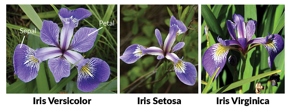
For this example, we will be working with the Iris Dataset. This data set is a real-world "toy" dataset that is often used to demonstrate concepts in data science. The iris dataset contains information about several flowers selected from three different species of iris: versicolor, setosa, and virginica.
For each flower, we have five pieces of information:
- The sepal length of the flower.
- The sepal width of the flower.
- The petal length of the flower.
- The petal width of the flower.
- The species of the flower.
The original iris dataset contains 150 observations. We will be working with a modified version of this dataset that contains 600 observations. The extra 450 observations were randomly generated to be similar to existing observations.
Load Packages
We will begin by loading three packages: Numpy, Pandas, and Matplotlib.
import numpy as np               # Numpy is used for performing vectorized operations.
import pandas as pd              # Pandas is used for data manipulation.
import matplotlib.pyplot as plt  # Matplotlib is used for plotting.
Load and Explore Data
The data is stored in the tab-separated file data/iris_mod.txt. We will use Pandas to load the data into a DataFrame called iris. We will then look at the first 10 observations in the DataFrame.
iris = pd.read_csv('data/iris_mod.txt', sep='\t')
iris.head(10)
We can use the Seaborn package to create a pairs plot of the the dataset.
import seaborn as sns
import warnings
warnings.filterwarnings("ignore")

%matplotlib inline
sns.pairplot(iris, hue="species")
plt.show()

The Goal
Our goal is to build a model that will allow us to predict the species of a newly observed flower for which we have measurements for sepal length, sepal width, petal length, and petal width.
We will consider two different models: a logistic regression model, and a decision tree model. We will use the package Scikit-Learn to construct, assess, and apply both of these models.
Scikit-Learn is a library that contains implementations of many machine learning algorithms, as well as useful tools for evaluatting models, processing data, and generating synthetic data sets. We will use this package extensively in this class.
Prepare the Data
The Scikit-Learn model-building API requires our data to be in a specific format. In particular, the features should be contained in a DataFrame or 2D Numpy Array, while the labels should be contains in a list or 1D Numpy array.
In the next cell, we create a feature array called X, as well as a label array called y.
X = iris.iloc[:,:4].values
y = iris.iloc[:,4].values

print(type(X))
print(type(y))

print("Shape of X:", X.shape)
print("Shape of y:", y.shape)
Splitting the Data
For reasons that we will explain in more detail later, it is important to split your data into three sets: the training set, the validation set, and the testing set.
- The training set is used to train the model. We will provide the training set to a machine learning algorithm as input, and the algorithm will generate a model as its output.
- The validation set is used to compare models. We will often wish to consider multiple different learning algorithms in a supervised learning task. Each algorithm will produce a single model that has been trained on the training set, and we will then compare the performance of the resulting models on the (previously unseen) validation set to help us select our final model.
- The testing set is used to assess the performance of our final model. This set is used only once, at the very end of the model building process.
When splitting your data into training, validation, and testing sets, it is import to first shuffle your data. We could do this manually, but fortunately, Scikit-Learn provides tools for creating a train/test/validation split.
from sklearn.model_selection import train_test_split

X_train, X_holdout, y_train, y_holdout = train_test_split(X, y, test_size = 0.20, random_state=1)
X_val, X_test, y_val, y_test = train_test_split(X_holdout, y_holdout, test_size = 0.50, random_state=1)

print('Training features:  ', X_train.shape)
print('Validation features:', X_val.shape)
print('Testing features:   ', X_test.shape)
print()
print('Training labels:    ', y_train.shape)
print('Validation labels:  ', y_val.shape)
print('Testing labels:     ', y_test.shape)
Model Building: Logistic Regression
Logistic regression is a classification algorithm that is designed to create linear boundaries between the different classes. In the next cell, we will use Scikit-Learn to create and train (or fit) a logistic regression model. We will then use the model to predict the species of a newly observed iris.
from sklearn.linear_model import LogisticRegression

m1 = LogisticRegression()
m1.fit(X_train, y_train)

x0 = [[4, 2.5, 2, 0.5]]
m1_pred0 = m1.predict(x0)
print(m1_pred0)
Model Building: Decision Trees
A decision tree algorithm employs a "divide and conquer" strategy to create a rules-based model for making classifications. We now use Scikit-Learn to create and train a decision model. As before, we will use the model to predict the species of a newly observed iris.
from sklearn.tree import DecisionTreeClassifier

np.random.seed(1)
m2 = DecisionTreeClassifier()
m2.fit(X_train, y_train)

x0 = [[4, 2.5, 2, 0.5]]
m2_pred0 = m2.predict(x0)
print(m2_pred0)
Comparing Models
For the single iris that we considered above, the two models agreed on the predicted species of the flower. It will not always be the case that two models agree in their predictions. Consider the following example.
x0 = [4, 2.5, 2, 0.5]
x1 = [5, 2.5, 6, 2.5]
x2 = [5, 2.5, 4.5, 0.5]
x3 = [6.5, 4, 5, 2]
xnew = [x0, x1, x2, x3]

print(m1.predict(xnew))
print(m2.predict(xnew))
We can use DataFrames to dispaly these predictions in a more readable format.
predictions = pd.DataFrame([m1.predict(xnew), m2.predict(xnew)])
predictions.columns = ['x0', 'x1', 'x2', 'x3']
predictions.index = ['Model 1', 'Model 2']
predictions
The models agree in their predictions for the first two flowers, but disagree in their prediction for the last two flowers. So which model should we use?
It would perhaps be instructive to see how well the models actually performed on the training data. To that end, we will calculate each model's accuracy on the training set. We will start with m1, the logistic regression model.
m1_pred_train = m1.predict(X_train)
m1_number_correct = np.sum(m1_pred_train == y_train)
print(m1_number_correct / len(y_train))
We will now calculate the training accuracy for the decision tree model, m2.
m2_pred_train = m2.predict(X_train)
m2_number_correct = np.sum(m2_pred_train == y_train)
print(m2_number_correct / len(y_train))
The logistic regression model achieved roughly 97% accuracy on the training set, which is good, but the decision tree model achieved 100% accuracy on the training set. That seems to indicate that the decision tree model is the better of the two. However, as mentioned before, we will always use the validation set to compare two models. So, we need to calculate the validation accuracy for each of the two models.
We could calculate the validation accuracies in the same way that we calculated the training accuracies above. However, our models actually come equipped with score() methods that will do this work for us. In the cell below, we will use the score() method to calculate training and validation accuracies for both of our models.
print("Model 1 Training Accuracy:  ", m1.score(X_train, y_train))
print("Model 1 Validation Accuracy:", m1.score(X_val, y_val))
print()
print("Model 2 Training Accuracy:  ", m2.score(X_train, y_train))
print("Model 2 Validation Accuracy:", m2.score(X_val, y_val))
Model 1 achieved a 95% accuracy on the validation set, which was slightly less than its training accuracy. Model 2, on the other hand, got an validation accuracy of 91.7%, despite getting perfect accuracy on the training set!
The behavior displayed by Model 2 is an example of overfitting. The model learns the nuances of the training set very well. Too well. It creates a model that performs very well on the data it was provided, but does not generalize well to new observations.
Since Model 1, the logistic regression model, has the better validation accuracy, we will select it as our final model. We conclude by using the testing set to provide us with a measure of the model's expected performance on new data once it is deployed.
print("Model 1 Testing Accuracy: ", m1.score(X_test, y_test))