import numpy as np
import matplotlib.pyplot as plt
As we saw in the previous lesson, logistic regression models (which consist of a single artifial neuron) always result in a linear decision boundary. While that might be appropriate for some problems, there are many problems for which a linear decision boundary will be insufficient. For those types of problems, we will need a more complex model. This can be achieved by stacking individual neurons together into an artificial neural network.
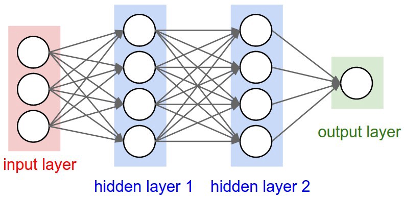
An ANN consists of many layers of neurons, which are processed in a specific order. There are three types of layers in an ANN: The input layer, one or more hidden layers, and an output layer.
The first layer, called the input layer, consist of the features being fed into the model. It contains one node for each feature being used, plus a single bias node.
The output of each node in the input layer is sent to each (non-bias) node in the first hidden layer. Every connection between any two pair of nodes in these two layers will have its own weight. The nodes in the first hidden layer process the inputs it recieves from the input layer, and send their outputs downstream to any subsequent hidden layers.
The last hidden layer will send its output to an output layer. This output layer could contain one or more neurons, depending on the type of task that the network is being used for.
We can build a neural network with as many hidden layers as we wish, and each hidden layer can have as many nodes as we would like. As a general rule, the more neurons that there are in a model, the more flexible that model is.

Example 1
The first neural network that we will build will be to tackle the following classification problem.
np.random.seed(887)
X = np.random.uniform(0,1,[300,2])
pB = 40*np.abs(X[:,0] - X[:,1])**4
pR = np.random.uniform(0,1,300)
col = np.where(pB < pR, 'r', 'b')
y = np.where(pB < pR, 0, 1)

plt.figure(figsize=(8,6))
plt.scatter(X[:,0], X[:,1], c=col, edgecolor='k', s=60)
plt.show()
Network Architecture
We will use keras to build a neural network with one hidden layer, containing four (non-bias) nodes.

Import Keras Modules
We will be using the Keras package to construct neural networks in this course. Keras provides a high-level API for building neural networks. It is built on top of TensorFlow, which is a library created by Google to efficiently perform matrix calculations.
We will now import some Keras modules that we will need to build our network.
from keras.models import Sequential
from keras.layers import Dense
from keras.optimizers import Adam
from tensorflow import set_random_seed
Construct the Network
We will now specify our network architecture by creating a class of type Sequential to represent our model. We will then add the necessary layers to our model.
np.random.seed(1)
set_random_seed(1)

model = Sequential()
model.add(Dense(4, input_shape=(2,), activation='sigmoid'))
model.add(Dense(1, activation='sigmoid'))
We can use the summary method to view a description of our model.
model.summary()
Compile the Model
Before we train the model, we need to specify what loss function to minimize, as well as what optimization method we will use to (hopefully) achieve that minimization. We can do this with the compile method of the Sequential class. We can also use compile to specify useful metrics other than the loss to be reported during training.
opt = Adam(lr=0.1)
model.compile(loss='binary_crossentropy', optimizer=opt, metrics=['accuracy'])
Training the Model
We will now train the model using the fit method. We specify values for the following parameters in the fit method below:
batch_sizerefers to the number of samples to calculate the loss on at one time. The weights will be updated after each batch. We will include the entire training set as our batch, but there can be advantages to using smaller batches. A single training loop will consider every sample in the data set, even if we are using multiple batches.epochsis the number of training loops to perform.verbosedetermines the amount of information displayed while training. Ifverbose=0, then no ouput is displayed. Ifverbose=2, then loss and any requested metrics are shown after each epoch. Settingverbose=1is similar toverbose=2, except that you will see a progress bar as well as execution time for each epoch.
h = model.fit(X, y, batch_size=300, epochs=200, verbose=2)
Analyzing Training Process
The output of the fit method contains a history attribute that we can use to visualize the changes in loss and accuracy during the training process.
plt.rcParams["figure.figsize"] = [8,4]
plt.subplot(1,2,1)
plt.plot(h.history['loss'])
plt.title('model loss')
plt.ylabel('loss')
plt.xlabel('epoch')

plt.subplot(1,2,2)
plt.plot(h.history['acc'])
plt.title('model accuracy')
plt.ylabel('accuracy')
plt.xlabel('epoch')


plt.show()
Visualiztion the Decision Region
I have written a function called plot_regions that can be used to plot the decision regions for classification problems with two features.
from ClassificationPlotter import plot_regions

plot_regions(model, X, y, cmap='bwr_r', fig_size=(8,6), keras=True)
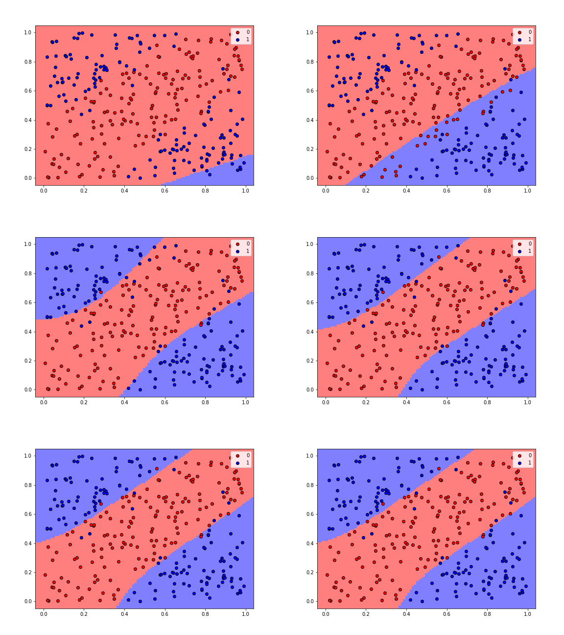
The gif below shows how the classification regions changed during the process of training.

Making Predictions
We can used the predict and predict_classes methods of our model to generate predictions for new observations.
Xnew = np.array([[0.2, 0.4], [0.2, 0.5], [0.2,0.6]])

np.set_printoptions(precision=6, suppress=True)

print('Estimated probabilities of being blue:\n', model.predict(Xnew))
print()
print('Predicted classes:\n', model.predict_classes(Xnew))
plot_regions(model, X, y, cmap='bwr', fig_size=(8,6), keras=True, display=False)
plt.scatter(Xnew[:,0], Xnew[:,1], marker="D", c='lime', edgecolor='k', s=100, zorder=3)
plt.show()
Example 2
We will now construct a neural network with a more complicated architecture to address the following classification problem.
from sklearn.datasets import make_circles

np.random.seed(1)
plt.figure(figsize=(8,6))
Z, w = make_circles(500, factor=0.25, noise=0.12)
w = (w+1)%2
plt.scatter(Z[:,0], Z[:,1], c=w, cmap='bwr_r', edgecolor='k')
plt.show()
Network Architecture
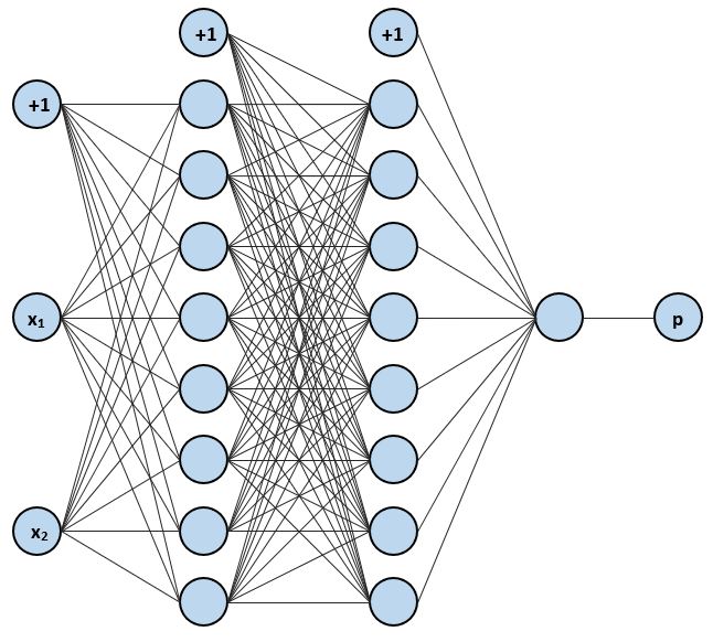
The network we will use for this problem will have two hidden layers, each containing 8 (non-bias) neurons.

Build, Compile, and Train the Network
We will now perform the same steps as before to build, compile, and train the network.
np.random.seed(1)
set_random_seed(1)

model2 = Sequential()
model2.add(Dense(8, input_shape=(2,), activation='sigmoid'))
model2.add(Dense(8, activation='sigmoid'))
model2.add(Dense(1, activation='sigmoid'))
model2.summary()
opt = Adam(lr=0.1)
model2.compile(loss='binary_crossentropy', optimizer=opt, metrics=['accuracy'])
h = model2.fit(Z, w, batch_size=500, epochs=50, verbose=2)
Analyzing Training Process
plt.rcParams["figure.figsize"] = [8,4]
plt.subplot(1,2,1)
plt.plot(h.history['loss'])
plt.title('model loss')
plt.ylabel('loss')
plt.xlabel('epoch')

plt.subplot(1,2,2)
plt.plot(h.history['acc'])
plt.title('model accuracy')
plt.ylabel('accuracy')
plt.xlabel('epoch')

plt.show()
Visualizing the Decision Region
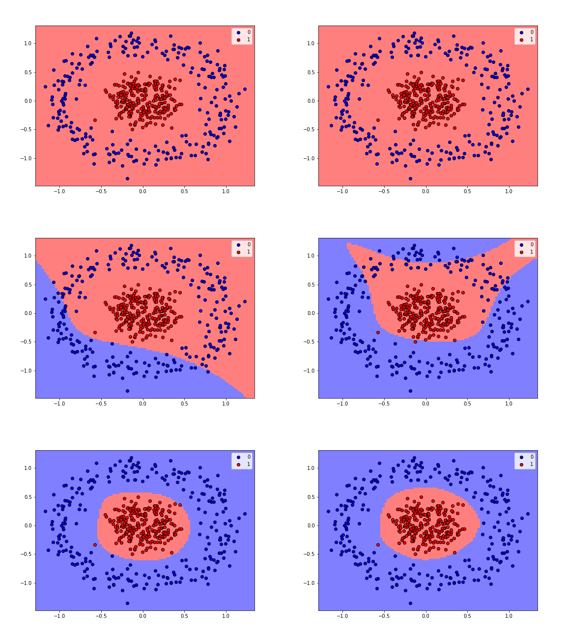
plot_regions(model2, Z, w, cmap='bwr_r', fig_size=(8,6), keras=True)

Generating Predictions
Znew = np.array([[0.5, 0.3], [0.5, 0.4], [0.5,0.5]])

np.set_printoptions(precision=6, suppress=True)

print('Estimated probabilities of being red:\n', model2.predict(Znew))
print()
print('Predicted classes:\n', model2.predict_classes(Znew))
plot_regions(model2, Z, w, cmap='bwr_r', fig_size=(8,6), keras=True, display=False)
plt.scatter(Znew[:,0], Znew[:,1], marker="D", c='lime', edgecolor='k', s=60, zorder=3)
plt.show()